|
Tutorial 3
Interpolation and integration |
Learning goals
|
Prior Knowledge |
 |
1 Objective
In this third tutorial, you will store the waterline data of the previous tutorial in a new object within the object Ships. You will perform linear and quadratic interpolation to obtain the relative width of unknown frames at the waterline. This will be checked with the exact solution, and the error is to be calculated. Some hydrostatic calculations will be performed: by numerical integration the waterplane area and the moment of inertia of this area are calculated. The stability GM will be calculated and compared to other ships using the least squares method.
Start
For this tutorial, the knowledgebase from tutorial 2 is used. You can either use your own (verified) knowledgebase, or download it here: [Tutorial 3 Start]
2 Creating a new object within a data object
The solution Waterline containing the shape of the dimensionless waterline, has been created in tutorial 2. In order to store this data and use it for further operations, the contents will be placed in a new object within the object Ships.
- In the class
Geometry, create a new object (i.e. a parameter of type Object) calledHull. As you need to store static data in this object, make sure it is determined by Value from Object/Database (as described in tutorial 2). - In the Workbase, select the object
Ships(under Dataset). In the Knowledge Browser, right click the parameterHulland select Parameter to Dataset (or press Ctrl+O or dragHulltotShips). The new object is now placed withinShips.
Let's add the content of the Waterline object in the Waterline solution to the object Hull.
- In the solution
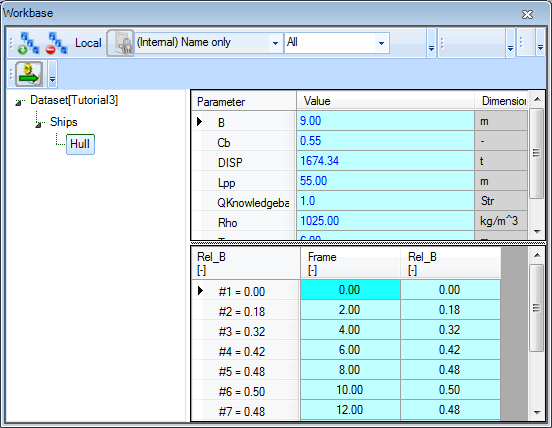
Waterline, in the tree of the Workbase, right-click on theWaterlineobject (so the tree node in the solution) and select All to Clipboard (or press F4). The Workbase Clipboard now pops up. Click on Preview. The contents of theWaterlineobject are now displayed. You temporarily have to use a workaround now, because the Paste function is not yet implemented. Press Ctrl+A followed by Ctrl+C to copy the contents to the Windows clipboard. Click Cancel and close the clipboard. No need to save the values in there. Then right-click on theHullobject in the Dataset and select Database Input or press Shift+F3. In the pop-up window that appears, select Use Editor and click Continue. In the window that appears next, press Ctrl+V to paste the data in the object. Click OK. Select Yes to All and click Continue.
When you are done, you will have a Ships object containing data in a Hull object. The Hull object should be part of the Ships object because the Ships object is the database entry point. And because you want to use all Waterline data as one set, it should be in one Hull object (or as a TeLiTab value as an alternative).
The workbase is full of solutions you'll not use anymore. So now first let's clean it up.
3 Interpolation
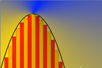
The relative width Rel_B at every frame was calculated directly using a polynomial formula. In reality, the waterline of a ship will be defined more likely by a number of points than by a formula. To obtain the width at a certain location, you should interpolate between these points. You can use the LININT() function to perform a linear interpolation.
- Add the following relation in
Top Goals/Undefined:
Intpol_Rel_B=LININT(@Hull,2,@Frame,@Rel_B,Frame)
- Make sure
Intpol_Rel_Bis dimensionless and determined by SYS: System/Equation.
The syntax of every intrinsic function in Quaestor is described in this documentation, see the functions overview. The syntax above means the following.
- The parameter
Inpol_Rel_Bwill be the linear interpolated dimensionless width at a desired frame number (Frame). @Hullis the object containing all the data you want to use for the interpolation.2is the number of dimensions in which the interpolation will take place.@Framemakes sure the columnFrameof objectHullwill be used as the parameter X in the interpolation.@Rel_Bmakes sure the columnRel_Bof objectHullwill be used as the parameter Y in the interpolation.Frameis the input parameter for which an interpolated value should be obtained.
When Quaestor calculates this function, it determines the value of Frame (which is user input). This value is then compared to the values of the given column for X (which is the column Frame of the object Hull), and an interpolated value for Rel_B with respect to the input Frame is assigned to the parameter Intpol_Rel_B. Notice that an @ is used to identify the data within the object.
- Run a solution for
Intpol_Rel_Busing the Process Manager and selecting theShipsobject. Make sure thatIntpol_Rel_Bis in the classTop Goals/Undefinedto see it in the Process Manager. The Process Manager is crucial here, as static data from theShipsobject should be used (which contains the objectHull). ForFrame, enter 3.20.
Quaestor should return 0.26 for Intpol_Rel_B.
To find out how accurate the interpolation is, let's introduce an Error parameter. The interpolated parameter uses static data from the object Hull, but you also defined the relative width analytically (the parameter Rel_B).
- Add the following relation to your
Top Goals/Undefinedclass:
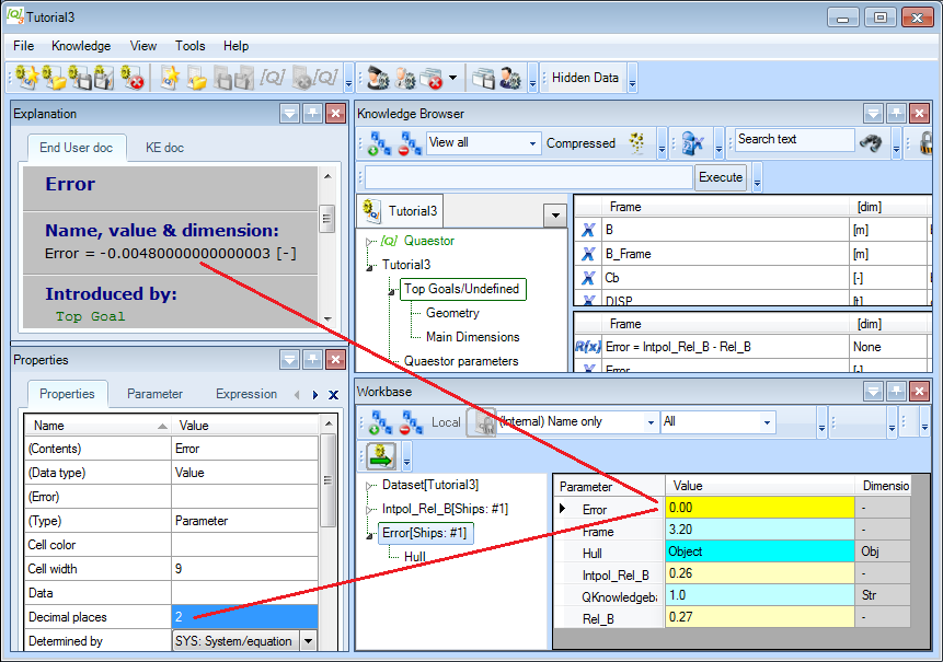
Error = Intpol_Rel_B - Rel_B
in which Error is a dimensionless SYS parameter.
- Run a solution for this parameter,
Intpol_Rel_Bwill be calculated by Quaestor automatically because it is required byError. Make sure you use the Process Manager to select theShipsobject as dataset. ForFrame, enter 3.20 again.
The solution in two-digit format (0.00) will be presented in the list of the Workbase. When you select this value, more digits are shown in the Explanation window.
You can change the number of decimal places presented in the Workbase by changing the value Decimal places in the Properties window.
For input values, the number of decimal places also defines the maximum accuracy accepted for this input. So, when you define B as having two decimal places, providing input with three will give a warning followed by rounding the provided number to two decimals.
- Change the number of decimals to 4 for
Error,Intpol_Rel_BandRel_Bto 4. - Change the relation (find the relation and press F2) for
Intpol_Rel_Bto
Intpol_Rel_B = DQUAD(@Hull, 2, @Frame, @Rel_B, Frame)
which uses the same data, but now performs a quadratic interpolation. It's not necessary to initialize existing solutions.
Editing relations was covered in tutorial 2. Remember that the use, syntax and examples of all Quaestor functions are available in the documentation: functionsoverview.
- Run the solution
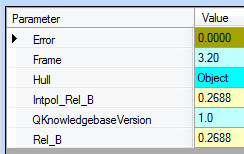
Erroragain with the same value ofFrame.
The error now turns out to be zero. This makes sense, as DQUAD is a quadratic interpolation method and this waterline is defined by a quadratic function as well.
4 Integration : waterplane area
By numerical integration, the waterplane area can be calculated. Therefore, the dimensionless length and width should be transformed to the real length and width. For the width you can use the existing relation for B_Frame, for the length in meters a new relation is needed.
- In the class
Geometry, add the following relation:
X = Frame/20 * Lpp
which is the position in meters along the longitudinal direction of the ship. By now you should know what proper dimension, reference and determined by value must be provided.
To calculate the waterplane area for a certain ship, Quaestor has to integrate the width with respect to X. The dimensionless width table is already present in your object Hull, so let's use it in the integration.
- In the
Top Goals/Undefinedclass, add the following relation:
Waterplane_Area = INTEGR(Hull(@X, @B_Frame, Lpp, B), 2, @X, @B_Frame, 2, 0, Lpp)
which is the waterplane area in square meters (m^2).
The syntax used here may seem a bit confusing at first.
First, take a look at the arguments after Hull. Data within the object Hull will be used in the integration, but yet it only contains dimensionless frame numbers and dimensionless widths. By putting (@X, @B_Frame, Lpp, B) behind it, you ask Quaestor to calculate X and B_Frame using data from within Hull, using Lpp and B from outside Hull and add all these parameters to the object Hull. You do actually use the object Hull as a function to calculate other parameters. This is a very powerful ability of Quaestor (see also QuaestorSyntax).
The arguments for the INTEGR function are as follows:
HULL(..)is the object from which data will be used, now containing the columnsXandB_frame2is the number of dimensions = always 2 using INTEGR.@Xrefers to the column that will be used as the parameter X in the integration:X@B_Framerefers to the column that will be used as the parameter Y in the integration:B_Frame2is the mode of integration, either Riemann (0), Trapezium (1) or Simpson (2). The latter is chosen here.0andLppare the values between which will be integrated.
- Run a solution for
Waterplane_Area, using the Process Manager.
The waterplane area is calculated for every variation in length and breadth of the ship.
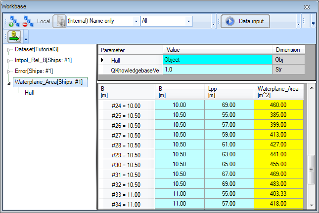
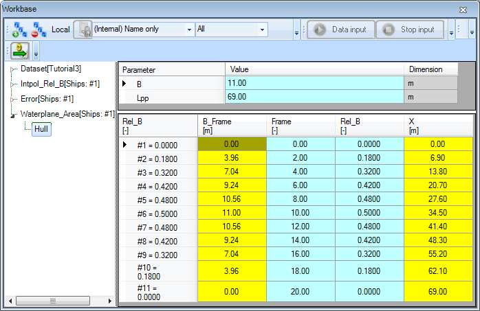
- In the
Waterplane_Areasolution tree, select the objectHull.
Because you solved a multiple case problem, the object has been used as function and reused for every case. Only the content of the last case calculated remains in the object. The columns X and B3_Frame are added to the object. These values are calculated for every case of Frame and Rel_B within Hull.
5 Calculating the stability
The initial stability (GM) of the ships can also be calculated using numerical integration.
- Add a new class, called
Stability, as sub-class ofGeometry. Add the following relation to this class:
GM = KB + BM - KG
The dimensions of all new parameters must be meters (m), and they are SYS parameters. Their relations follow. GM is a Top Goal and should be moved to Top Goals/Undefined.
- In the class
Stability, enter the following relations.
Distance between keel K and center of buoyancy B, select KB , right-click and select New Relation... (or press Ctrl+N). By selecting KB it is automatically presented as left side part of the relation:
KB = 0.7 * T
Distance between keel K and center of gravity G, KG, in meters:
KG = 0.8 * T
Distance between center of buoyancy B and metacenter M, BM, in meters:
BM = Moment_of_Inertia / (DISP * 1000/ Rho)
Third power of the width at a specified frame number in m^3:
B3_Frame = B_Frame^3
Moment of inertia of the waterplane area in m^4:
Moment_of_Inertia = 1/12 * INTEGR(Hull(@X, @B3_Frame, Lpp, B), 2, @X, @B3_Frame, 2, 0, Lpp)
Note that the syntax of the moment of inertia relation is similar to that of the waterplane area relation.
Do not forget to provide all dimensions and references, and change the Determined by fields to SYS: System/equation.
- Add
@RANGEALLOWEDto parameterDISP(Parameter tab, Data field of Properties window). - Run a solution for the initial stability
GMof every possible ship, by selecting theShipsobject andGMas task in the Process Manager. Press Next repeatedly until the text on the button turns to Data input again and the solution is completed. - In the
GMsolution tree, select the objectHull.
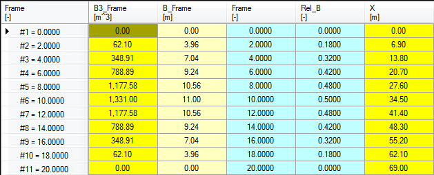
If the object Hull in the solution is now opened again, you'll see that, like for the waterplane area, the columns X and B3_Frame are added to the object, whose values are calculated for every case of Frame and Rel_B within Hull. Note that the parameter B_Frame is also added, as it is used to calculate B3_Frame. Again, only the values of the last ship (last input case) are stored in the object.
6 Comparing the stability to other ships
Finaly, let's compare the obtained values for GM to other ships. Data of the GM value for a certain ship length is available, so we only have to compare them. You can use the least squares method to obtain an average GM value for a certain length, using the data of some other ships.
- Add the following new relation to your
Top Goals/Undefined:
GM_Check = LEASQ(TEXTITEM$(1), 2, "L", "GM", Lpp, 2)
GM_Check is in meters.
- Enter the following text in the Expression Data field in the Expression Editor of the relation
GM_Check:
TEXTITEM1 =
|0
3 "ExampleShip" "L" "GM"
"1" 1 70 0.6
"2" 2 75 0.7
"3" 3 60 0.5
"4" 4 80 0.9
"5" 5 75 0.55
"6" 6 60 0.6
"7" 7 55 0.8
"8" 8 65 0.75
"9" 9 72 0.6
"10" 10 80 0.56|
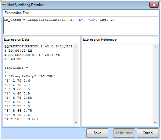
The LEASQ interpolation function now returns an average GM value in meters for a certain Lpp. The syntax TEXTITEM$(nr) is often used in Quaestor, and refers to a template, text item or TeLiTab in the Data slot of the Expression Editor. In this way, data that is not included in the knowledgebase but is only used in a particular function (as in our relation) can be used.
Note that the syntax of the relation uses TEXTITEM$(nr), but in the data slot the syntax TEXTITEM1= is used. The TeLiTab is written between two | characters. Multiple textitems can be available in a relation (TEXTITEM$(1), TEXTITEM$(2) .. TEXTITEM$(n)).
Please note that "the devil is in the detail". Small errors in your syntax will always be a problem for software such as Quaestor. Therefore, keep checking the correctness of your syntax.
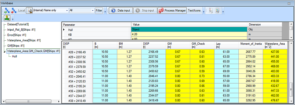
- Run a solution using the Process Manager. Select
Waterplane_Area,GMandGM_Checkas goals. Again, press Next until the solution is completed.
You can select several goals at once!
To browse through results, it might be convenient to maximize the workbase window. The result of the last solution should look like this:
7 Check
You can verify your results by comparing it to [Tutorial 3 Finished]
Overview
Content Tools