Using Quaestor objects
Quaestor employs a powerful ‘parameter’ concept, i.e. a parameter can be a numerical attribute like length, mass and cost, but also nominal (string) values can be dealt with such as color, client name or contents of program output files.
Apart from the numerical and nominal parameter type, Quaestor uses the Object type. A Quaestor object is a parameter which has a set of parameters with values as value, either static (only data, e.g. a speed-power curve or a list of components) or dynamic, i.e. a computational model (input and output) fulfilling the role of function or subroutine in an assembled model (a Solution in the Quaestor Workbase).
1 Objects as Dynamic Function
The Quaestor object is just a frame in the knowledge base such as a parameter, relation or constraint. For example PowerCalc
In a Relation, PowerCalc can be used as if it were an intrinsic function like SIN(), SELECT() etc. as in the following example:
Power = PowerCalc(@Power, @Method:"Savitsky", @Speed:Vdes, L, B, T, D)
In this example PowerCalc represents the object (container) of a computational model that will compute Power on the basis of the values of Method="Savitsky", Speed=Vdes and the actual values of L, B, T and D. The @ character indicates that the parameter should exist in the PowerCalc object, the first parameter after the opening bracket (@Power) is the top goal of the PowerCalc object, @Speed:Vdes means that Speed in PowerCalc should get the value of Vdes. Values of L, B, T and D are required but not unique to this object and therefore requested as normal parameters and should be available "above" or outside the object. See also Quaestor syntax for more detail.
The following modeling rules apply:
- If the model in PowerCalc needs data that is not in the argument list, it is either requested to the user in the object or inherited from the models top level.
- If input is provided manually, the value is placed in the models top level. This implies that the value is available (can be inherited) by all objects in the model.
- If the parameter has the @LOCAL attribute in its data slot, the value is stored in the object and is only available to that object.
In the above example, the PowerCalc() function returns the value of Power that is computed by the PowerCalc model that is assembled for the top goal Power.
The object PowerCalc created by evaluating the above relation is reusable and extensible: it is possible to request other goals from the same object instance, for example the rotation rateRevs:
N = PowerCalc(@Revs, @Method:"Savitsky", @Speed:Vdes, L, B, T, D)
If this relation is evaluated later than the earlier one, and Revs is not yet computed, Revs is added as top goal to the object after which the object attempts to add the necessary relations to its model and will compute its value.
If another relation is evaluated that evaluates Power with other input, the calculation in PowerCalc is redone. Only the last results in the object are maintained in the solution. Use the @MULTICASE attribute to force the object to save all its values. Realize that this might require more memory and will let your project files grow significantly.
The table below lists the return type for every Left side, Goal type, List/Table and Return type combination, along with an example. So if the left side is a String the return type is a Telitab, when the left side is a value the return type is a pointer to an object, except when the goal type is a list of values, then the return type is a value. Assigning a pointer to a value parameter is useless as it can not be used. It only makes sense in a function call. Then it is used implicitly. However the expression editor does not support this yet. At the moment it is possible to define an expression that will assign a pointer to a value parameter. This will be solved in a future release. However, the case when the left side is a value and the goal type is a table of values can only be detected run-time, and can therefore not be prevented in the expression editor.
Left side | Goal type | List / Table | Return type | Expression | Goal | Input | ||
|---|---|---|---|---|---|---|---|---|
| Value | Value | List | Value | Y = DataObject(@Y, @X:STR$(Xmin)+"(0.1)"+STR$(Xmax)) | Y = X^2 | Xmax = 3 | Xmin = 3 | |
| Value | Value | Table | Pointer to DataObject | Y = DataObject(@Y, @X:STR$(Xmin)+"(0.1)"+STR$(Xmax)) | Y = X^2 | Xmax = 3 | Xmin = 1 | |
| Value | String | List | Pointer to DataObject | Y1 = DataObject(@D$, @X:STR$(Xmin)+"(0.1)"+STR$(Xmax)) | D$ = STR$(2*X^2) | Xmax = 3 | Xmin = 3 | |
| Value | String | Table | Pointer to DataObject | Y1 = DataObject(@D$, @X:STR$(Xmin)+"(0.1)"+STR$(Xmax)) | D$ = STR$(2*X^2) | Xmax = 4 | Xmin = 3 | |
| Value | Telitab | List | Pointer to DataObject | y2 = DataObject(@C#) | C# = TELITAB#(0,A,B) | A = 1 | B = 1 | |
| Value | Telitab | Table | Pointer to DataObject | y2 = DataObject(@C#) | C# = TELITAB#(0,A,B) | A = 1(1)10 | B = 2(2)20 | |
| Value | Object | List | Pointer to ChildObject | y3 = DataObject(@ChildObject, @X:STR$(Xmin)+"(0.1)"+STR$(Xmax)) | ChildObject(@Y, X) | Y = X^2 | Xmax = 3 | Xmin = 3 |
| Value | Object | Table | Pointer to DataObject | y3 = DataObject(@ChildObject, @X:STR$(Xmin)+"(0.1)"+STR$(Xmax)) | ChildObject(@Y, X) | Y = X^2 | Xmax = 4 | Xmin = 3 |
| String | Value | List | Telitab | Y$ = DataObject(@Y, @X:STR$(Xmin)+"(0.1)"+STR$(Xmax)) | Y = X^2 | Xmax = 3 | Xmin = 3 | |
| String | Value | Table | Telitab | Y$ = DataObject(@Y, @X:STR$(Xmin)+"(0.1)"+STR$(Xmax)) | Y = X^2 | Xmax = 3 | Xmin = 1 | |
| String | String | List | Telitab | Y1$ = DataObject(@D$, @X:STR$(Xmin)+"(0.1)"+STR$(Xmax)) | D$ = STR$(2*X^2) | Xmax = 3 | Xmin = 3 | |
| String | String | Table | Telitab | Y1$ = DataObject(@D$, @X:STR$(Xmin)+"(0.1)"+STR$(Xmax)) | D$ = STR$(2*X^2) | Xmax = 4 | Xmin = 3 | |
| String | Telitab | List | Telitab | y2$ = DataObject(@C#) | C# = TELITAB#(0,A,B) | A = 1 | B = 1 | |
| String | Telitab | Table | Telitab | y2$ = DataObject(@C#) | C# = TELITAB#(0,A,B) | A = 1(1)10 | B = 2(2)20 | |
| String | Object | List | Telitab | y3$ = DataObject(@ChildObject, @X:STR$(Xmin)+"(0.1)"+STR$(Xmax)) | ChildObject(@Y, X) | Y = X^2 | Xmax = 3 | Xmin = 3 |
| String | Object | Table | Telitab | y3$ = DataObject(@ChildObject, @X:STR$(Xmin)+"(0.1)"+STR$(Xmax)) | ChildObject(@Y, X) | Y = X^2 | Xmax = 4 | Xmin = 3 |
2 Object as Pseudo-Intrinsic Functions
A second way to use the Quaestor object is to define a Function.
You need:
- to create a generic relation for you function;
- to define the general syntax for you function;
The first is done in the normal way. The second is done by using the New Parameter/Function menu option in the Knowledge Browser and providing the function definition:
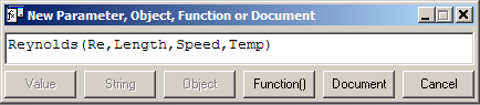
In this example a pseudo intrinsic function is created to calculated the Reynolds number.
Reynolds is the Quaestor object, Re the top goal for the calculation to be performed with in the Reynolds instance and Length, Speed and Temp are the input arguments.
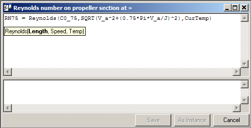
Relations should be available to compute Re on the basis of Length, Speed and Temp, as in Re=Speed*Length/Nu and Nu=f(Temp). This form of function definition will present theReynolds() function in the expression editor as if it were a Quaestor intrinsic function like SIN() or SELECT(). Any values or parameter can be used to fill in on the locations of Length, Speed and Temp, as in the following example:
RN75=Reynolds(C0_75,SQRT(V_a^2+(0.75*Pi*V_a/J)^2),CurTemp)
RN75 represents the Reynolds number of the propeller blade section at 0.75R in which:
Length = C0_75
Speed = SQRT(V_a^2+(0.75*Pi*V_a/J)^2)and
Temp = CurTemp
Please note that the above could also be written in the first method as follows:
RN75 = Reynolds(@Re, @Length:C0_75, @Speed:SQRT(V_a^2+(0.75*Pi*V_a/J)^2), @Temp:CurTemp)
This example shows that the pseudo intrinsic way of defining functions is an elegant way to use Quaestor objects, in particular since the functions that are defined in this manner are presented in the Quaestor/Functions overview in the browser.
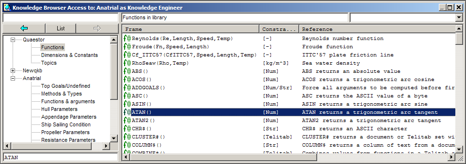
It should be noted that the pseudo intrinsic functions presented in the Functions class of the Quaestor tree node, belong to the knowledge base last in focus before entering the function list. The expression editor recognizes these functions and presents the arguments one by one.
The pseudo intrinsic function can be re-used for other input but cannot be used to compute other values as the expression editor only allows the argument sequence that is predefined in the function definition. Again, only the last results in the object are maintained in the solution.
3 Objects Relations
A novel and powerful form of using Quaestor objects is as Object Relation. It allows the creation of basic configurators, the Taxonomy approach is an improved implementation.
The following example shows how this works.
By introducing the following list of relations in a new knowledge base, a miniature configurator is obtained:
Relation 1:
Ship(@Decks,@Bulkheads)
Relation 2:
Decks(@Deck)
Relation 3:
Deck(@Area, @ID$)
and put "@ASKORDER:Nr" in the data slot of Deck on a new line
Relation 4:
Bulkheads(@Bulkhead)
Relation 5:
Bulkhead(@Area, @ID$)
put"@ASKORDER:Nr"in the data slot of Bulkhead on a new line
Relation 6:
Area = L*B
put @LOCAL attribute in the data slots of L and B
Relation 7:
ID$ = CUROBJECT$(1)
Do not forget to provide the parameters dimensions in the Frame viewer, top right.
Include Nr in the knowledge base with the New Parameter/Function menu option as Value and put @LOCAL in its data slot.
When creating the relations, Quaestor may ask whether parameters are of the Object type. Obviously, Decks, Deck, Bulkheads and Bulkhead are objects, Area is not an object but a value. ID$ is automatically made into a string due to the $ suffix.
You see that the relations in object form do not have a left hand term such as in Area = L*B. If an object such as Ship or Deck is created in this manner, they are automatically provided with the @LOCAL attribute. Non-object parameters that are used as goal or input arguments in the function do not necessarily need the @LOCAL attribute, as in the case of ID$ and Area, because they are automatically instantiated in the object. L and B, however, are not given as function arguments but introduced into the object by the relation Area = L*B. If L and B are not @LOCAL, the input is saved in the solution's top level. The result will be that all decks and bulkheads will have the same L and B since these can be found higher up in the model.
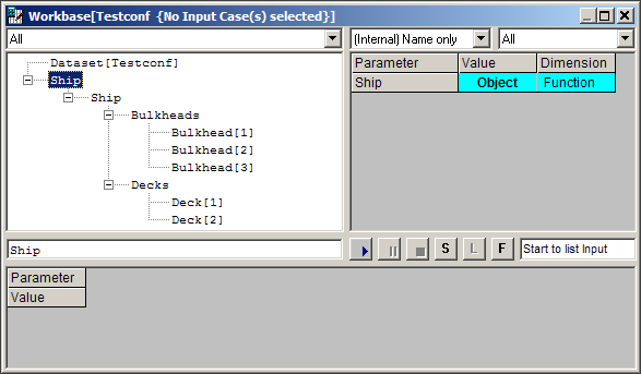
If Ship is selected as top goal (by double clicking on the Ship parameter) and the dialogue is started, you are requested to provide the number of decks, their respective L and B and the same for the bulkheads.
The result you get after finishing the dialogue is an object model of Ship containing all decks and bulkheads.
4 Object Initiation and Access
Next to the direct use of Quaestor objects as functions, it is possible to refer and use value from these objects in expressions. This in an implicit way of using the objects because they have to be created when you want something it contains.
Simply create a new knowledge base with the following relations:
QuadraticCurve(@Y,@X:"0(1)20")
Y = X^2
Couple the QuadraticCurve object to the relation Y = X^2 through the Constraint Connect menu option in the Knowledge browser:
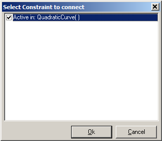
This makes that Y = X^2 is only valid within an instance of QuadraticCurve.
Enter the next relation:
Y = DQUAD(@QuadraticCurve, 2, @X, @Y, X)
Select Y as top goal and enter a value 3.5 for X. You will see that the QuadraticCurve object is created in the solution and you will get a result of 12.25.
Enter an additional relation that selects the third Y value from the QuadraticCurve object:
Y_3 = QuadraticCurve.Y.3
Select Y_3 as top goal will yield a result of 4.0.
Alternative 1:
A similar result can be achieved with only two relations.
Introduce into an empty Quaestor the relations:
Y = DQUAD(@QuadraticCurve, 2, @X, @Y, X)
Y = X^2
Connect this relation to the QuadraticCurve object as is done above.
X must be provided with the @LOCAL attribute in its dataset, since it is to be used both in the solution top level and in the QuadraticCurve level.
QuadraticCurve must be provided with the OBJ attribute in the Determined By property:
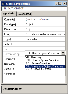
In this case QuadraticCurve is introduced in the model by the first relation. And the OBJ attribute makes it into a non-computable object which will create the X and Y values through the @X and @Y arguments in the relation (the @ stands for parameter presence in the object).
If you ask for Y and give respectively X=6 (in the solution level) and X=1(1)10 (in the QuadraticCurve level) you will get the obvious result of 36.
Alternative 2:
Yet another way to create objects is illustrated by the following relations:
Z=QuadraticValue.Y
Y=X^2
Ask Z and give X=3 and you will get 9 as result. The QuadraticValue object in the solution contains the calculation with the Y=X^2 relation.
See the Quaestor syntax for all the specific syntax for objects.
Overview
Content Tools